Color Quantization
Can the color content of an image be simplified? In other words, can you create a map from all colors in a picture to a limited subset with tens of members? This amounts to finding the densest regions of the pixels distributed through a color space and replacing them with a representative value. We can pose this as a clustering problem, although it is essential that no assumptions be made about the scene, particularly not the number of clusters. We can also treat it as a minimization of the difference between the simplified and actual colors, summed over all pixels. In either case the central idea is the population of pixels per color, which determine where to place the limited colors and the extent of the mapped regions.
Let us work in a color space that separates luminance from color, like YCrCb (YUV) or the CIE LA*B* spaces. There are then two color axes and, with 8 bit channels, a 256x256 plane of all possible colors in an image. Build a histogram from the image, where each bin in the plane counts the number of pixels with that color. We can view this as a terrain map, where the peaks are the most common colors and the massifs that surround them the similar regions. The center of mass of the region, or the average color weighted by the bin counts, is the best representative value that minimizes the error over the region. A watershed algorithm is a good way to find the local maxima and their neighborhood because we have a discrete grid and not a functional form for numeric analysis. The watershed is an inverted waterfall, where we look for peaks instead of basins and water drains away instead of collecting, although in both cases it flows along the greatest gradient or height difference (ignoring the different distance to diagonal neighbors).
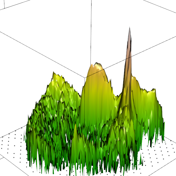
Original RGB image and histogram in Cr-Cb color plane, displayed in 3D relief (left, with the log of the count on the z axis) and as a topo map (right). Note that the 3D map is rotated 90 degrees counter-clockwise to better see the ridge.
In the watershed algorithm you sort points (bins) by decreasing height (count) and then work down the list, either assigning a pixel to its highest neighbor (maximum gradient) or marking it as a boundary between two drainage areas or registering it as a new peak if neither applies. Our implementation pre-computes the gradient. At each bin it examines the neighbors, marking those with the greatest height as the direction of inflowing water. There may be more than one, which might mean it lies on a boundary (or maybe not, depend on the topography). We marks neighbors at the same height as on a flat or plateau. In a second pass, for all bins with a single inflow and not on a flat, we mark the outflow in the neighbor: when water reaches the neighbor, it must also flow into the pixel. On a plane a bin has eight neighbors, so these markers can be bit-encoded and processed with logical operators. The calculations are local and can be done in parallel at each bin, instead of scanning all neighbors as the watershed algorithm works through the sorted list, which is a serial operation.


Flows between bins and highest neighbor(s). Inflows (left, green) are stored in bin with arrow. Outflows (middle, brown) are stored in source bin and only point to neighbors with one inflow; the algorithm can automatically follow these once the source is assigned. Flats (right, blue) mark neighbors with same counts.
For each bin in the sorted list, the algorithm first checks if all inflowing neighbors (when there's more than one) belong to the same drainage area; if so, the bin belongs to it. If the bin is on a plateau then it makes the same check on all inflowing neighbors to the flat, and only if there's one source the whole flat can be marked as part of the drainage. If for either the bin or the flat there are no inflows, then it is a new peak, which the algorithm registers and marks. If a bin or flat has inflows from more than two peaks, then it is a boundary and left unassigned (which also blocks the same source check for neighbors). For any bins assigned at this time, the algorithm then follows all outflow markers, assigning them to the peak's drainage area. This can continue in a chain. When done with the list, the algorithm makes a second pass to assign border bins to the highest neighboring peak, or closest drainage if in the middle of a large plateau.
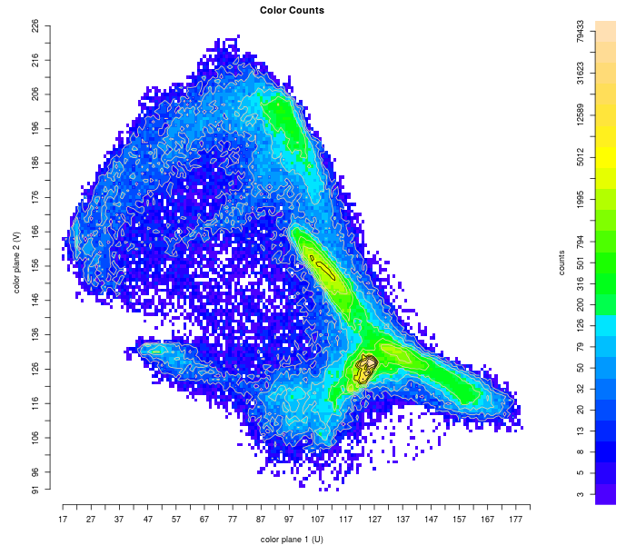
The watershed may contain insignificant peaks that we will want to eliminate. Like the AMC and ADK 4000 Footer rules, "insignificant" is arbitrary. Here a subsidiary peak is one with too small a drainage (number of bins in area), or too small a volume (total count in all bins), or too shallow a saddle to an adjacent peak (height difference from peak to highest boundary bin). These should be merged into a neighbor. We also find problems with massifs with long, gentle flanks. The drainage areas extend far from the peak, and although there may not be many pixels in these distant areas because the height/counts are low, the difference is large enough to cause artefacts in reconstructed images. Handling this case is complicated. If drainage areas are limited to a distance r from the center of mass, it can leave a mass of newly unassigned bins with an awkward shape. We can use the midline of the mass to place covering circles of radius r, assuming the width is no more than twice r. The midline is a skeleton equidistant from the edges of the mass, and in our implementation is marked during successive erosions. Before each the algorithm looks for single bins or 2x2 blocks that will be removed from two sides, that have in other words two out-of-mass (eroding) neighbors that are separated by in-mass. When done this can leave a few artefacts, including whole 2x2 blocks that can be thinned, checkerboards, and dangling bins, so a cleanup pass is needed. The number of the erosions when the midline is marked equals its distance from the edge.
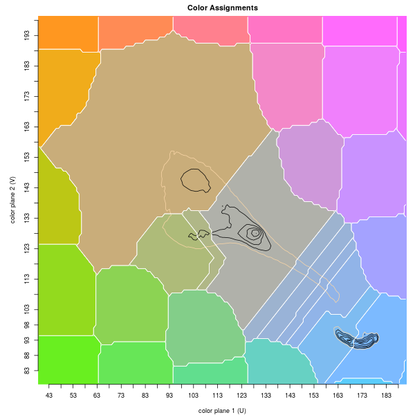
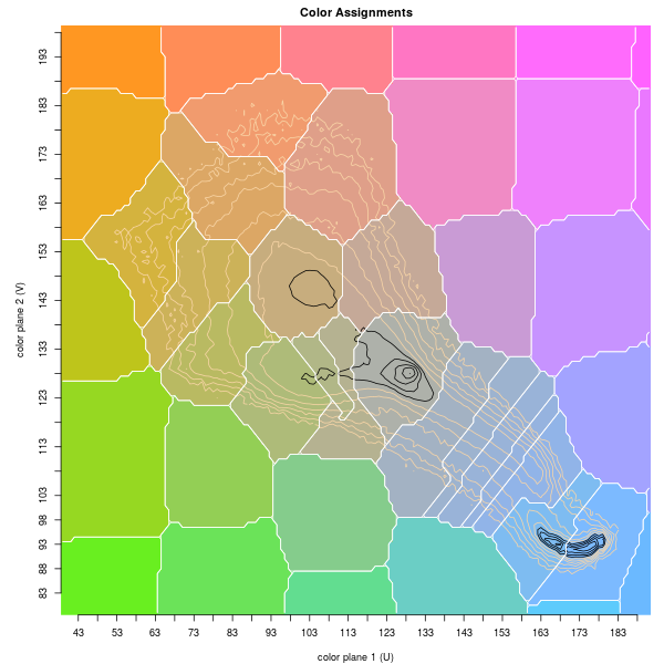
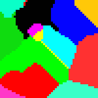
Histogram of problematic image. Bottom left quantization shows large flanks around top left and central peaks, mapping to brown and grey. Limiting distance from peak, shown in bottom right, restores colors.
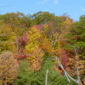
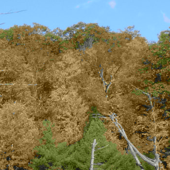
Effect of large flanks. Original image on left, color-quantized with large flanks in middle showing red and yellow replaced by brown, and color-quantized after limiting distance on right.
Placing covers occurs in two steps. First, we look at points set back about r from the edge (plus or minus a few, checking from smaller to larger), and calculate how much of the mass a circle of radius r would cover and what fraction of the circumference is occupied by the mass. If the coverage is high enough, and using a lower threshold if not much of the circumference is occupied, then set the cover by creating a mock peak and blocking other midline points where a second cover would overlap the current by 15%, which happens at 1.5r. The idea behind the lower threshold is that we want to encourage placement at "pointy" ends of the mass. In the second step we work through the remaining midline points, picking those with a large enough coverage (excluding bins covered in the first pass) while minimizing the overlap with one another. When done, we then assign bins to the nearest mock peak.

Bins with non-zero counts that are far away from the peak (left, from the distribution above), and the midline and covering circles that create new quantization areas (right). The second pass covers are slightly darker.
This will still leave some bins unassigned. In principle we can put them in the nearest drainage, with ties resolved to the highest source, but we must also make sure that the drainage areas are contiguous; they cannot be disjoint. This requires a region growing strategy, expanding by one bin in every direction with each pass until all bins are assigned.
Color Quantization via Watershed
-
count, smooth, and adjust histogram
-
pre-calculate maximum gradient neighbors (inflows), reverse gradients (outflows), flats
-
sort bins in descending count order
from highest to lowest, assign bins
if all inflows from bins assigned to same peak and no same-height neighbors, to that peak
else if on a plateau and all inflows from bins assigned to same peak, to that peak
else if not adjacent to two or more different peaks, to a new peak
then follow outflows from bin(s) just assigned, adding to peak's drainage area
-
assign boundary (unassigned) bins to nearest peak, or highest if tied distance
-
merge subsidiary peaks (either small in area or volume or with shallow saddles to neighbors)
limit extent of drainage area and cover distant bins with mock "peaks"
mark distant bins
find midline through mass, then distance along
place mock peaks along midline set back a distance from the edge according to coverage
place mock peaks along midline in interior of distant bins to maximize coverage
convert mock peaks into new regions and assign bins
-
assign all remaining pixels, from Step #7 and those adjusted in Step #1, by region growing drainages
-
create square grid in periphery and fill in the color plane
-
bob tails, thin whiskers of drainage areas winding between other areas
The complete algorithm contains extra pre- and post-processing steps.
In Step #1, it's useful to run a small 3x3 or 5x5 averaging filter over the histogram counts and rounding fractions. This smooths the surface, reducing subsidiary peaks and making gradients more uniform; the rounding reduces noise by creating larger flats. We also clip counts below a small threshold to zero, to improve the edges of massifs and prevent large, almost flat skirts. These bins are assigned peaks in Step #8, alongside the distant bins not yet covered. In some images with little color content, perhaps a winter scene or one filled with concrete objects, the greyscale or colorless point will have a substantial peak with a large drainage area that will cover weak colors. We can zero bins in a small radius about the point to force the creation of a few peaks with light colors. Other ideas to reduce noise are to make one or two dilation passes to smooth the edges, or to fill in zero count bins that are mostly surrounded. However, we find the averaging filter is sufficient.
The source image will not have all 256x256 colors, and some bins will be empty. New pictures of the same scene will contain some of these colors, either from illumination changes or noise, and we need to include them in the mapping. In post-processing Step #9 we create a coarse, rectangular grid of mock peaks to fill in the periphery, the bins with zero counts. Tile the color plane with the grid and calculate the number of non-zero pixels (ie. that have already been assigned) under each grid point. Drop points that aren't needed or shift away those near assigned areas. We do this by counting the assigned bins above and below, left and right of the grid point and shifting them away proportional to the count; their neighbors then move in turn so they have equal spacing in either direction. We then use region growing from the seeds to cover the zero count bins.
The region growing of the last two steps can produce one more artefact to clean up. A region can grow a whisker or "tail" of single bin width that winds between two others. To remove the tails in Step #10 we repeatedly eliminate the endpoint, assigning it to the most common neighbor.
Long tail just one pixel wide (left, in yellow) is bobbed (right).
Some typical values of the magic numbers sprinkled through the discussion above are
|
Step |
Parameter |
Value |
|
1 |
size of averaging filter |
3x3 |
|
1 |
adjust count: zero if below threshold |
5 |
|
6 |
minimum area (bins) in drainage area |
10 |
|
6 |
minimum volume (counts) in drainage area |
500 |
|
6 |
minimum height of peak off saddle |
5 |
|
7 |
maximum extent of drainage from center of mass |
12 |
|
7 |
minimum fraction cover area over mass for any edge point |
2/3 |
|
7 |
minimum fraction cover area over mass if "pointy" edge |
1/3 |
|
7 |
maximum fraction circumference w/ non-zero pixels for "pointy" edge |
1/4 |
|
7 |
minimum fraction cover area in pass 2 |
1/4 |
|
9 |
distance between peripheral grid points |
30 |
Quantization produces a map on the color plane, with a peak assigned to each color pair. To apply the mapping, replace each pixel's color with the center of mass of the peak, keep the pixel's luminance, and convert to the display color space.
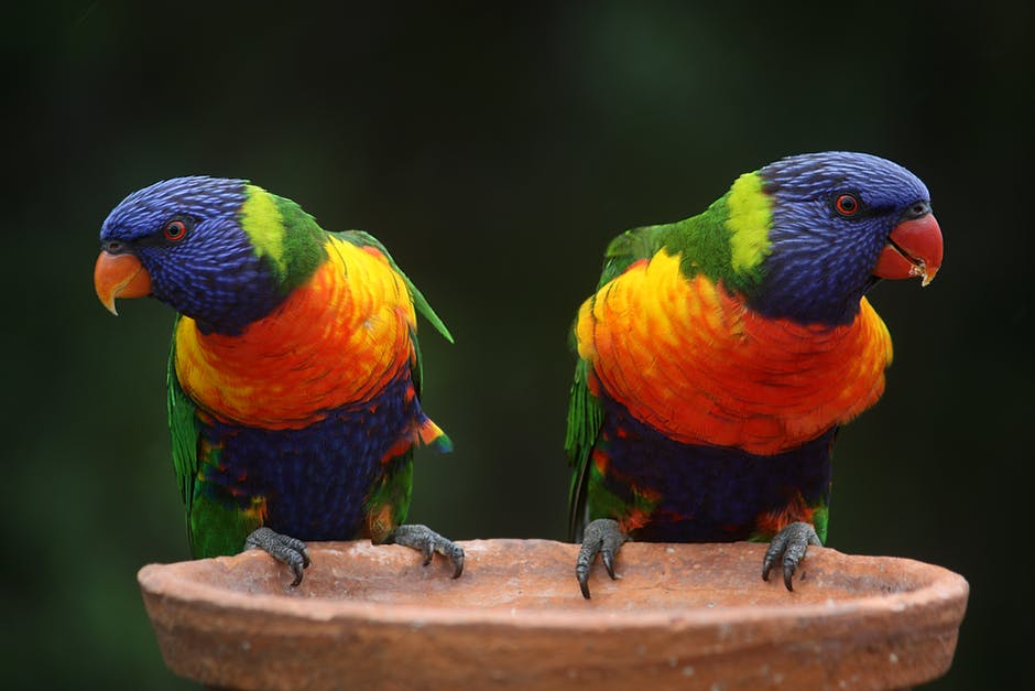
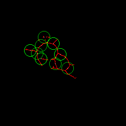
On the picture with the parrots we find 20 peaks, plus another 58 created for the fill-in grid. The largest peak is the greyscale point, with ID 1. It dominates the landscape, with the peak seventeen times higher than the next and with four times the volume in the region. The next highest lies to the northwest; it has a reddish brown color from the bowl. We can view the quantization areas in the color plane with the topographic contours superimposed and areas shaded by the center of mass color at a nominal luminance.
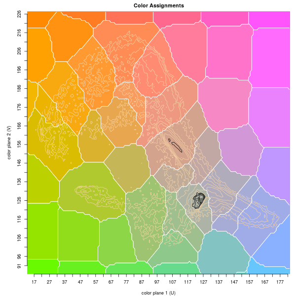
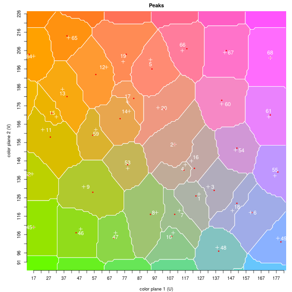
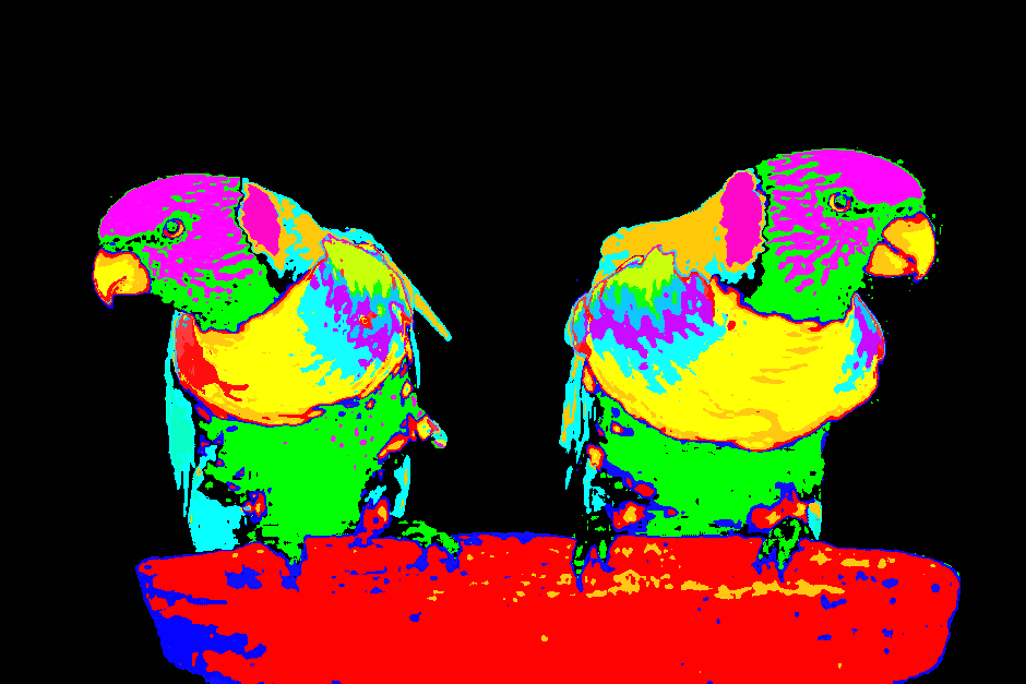
Color quantization areas of parrots image. Map on left shows areas and replacement colors atop topo contours. Map on right shows peak IDs and location (crosses) and centers of mass (red dots). Bottom image has peak assignments; coloring is random.
After applying this map the reconstructed image shows good performance, with a few typical artefacts. Most obvious are the blotches in the basin. This happens when the drainage area is too large and the natural color lies too far from the peak. We also find in the basin that greyish areas on the inner rim have been filled in with the overall basin color. A larger area on the bottom left of the basin's outside edge has mapped to a darker grey and a hard edge. Both of these artefacts come from limiting the number of colors. On the parrots the most visible changes are steps caused by the quantization of gradients, on the throat of the left bird, the beak of the right, and on its breast. Pixels on either side of the step are assigned to different peaks, although in reality the change is more subtle. Roughing the edge, dithering these pixels, or interpolating between the two peaks, would make the transition smoother. The final difference we note is the loss of texture on the right parrot's breast, where the quantization loses subtle shading. Although not present in this image, another artefact we see is color noise at sharp edges.
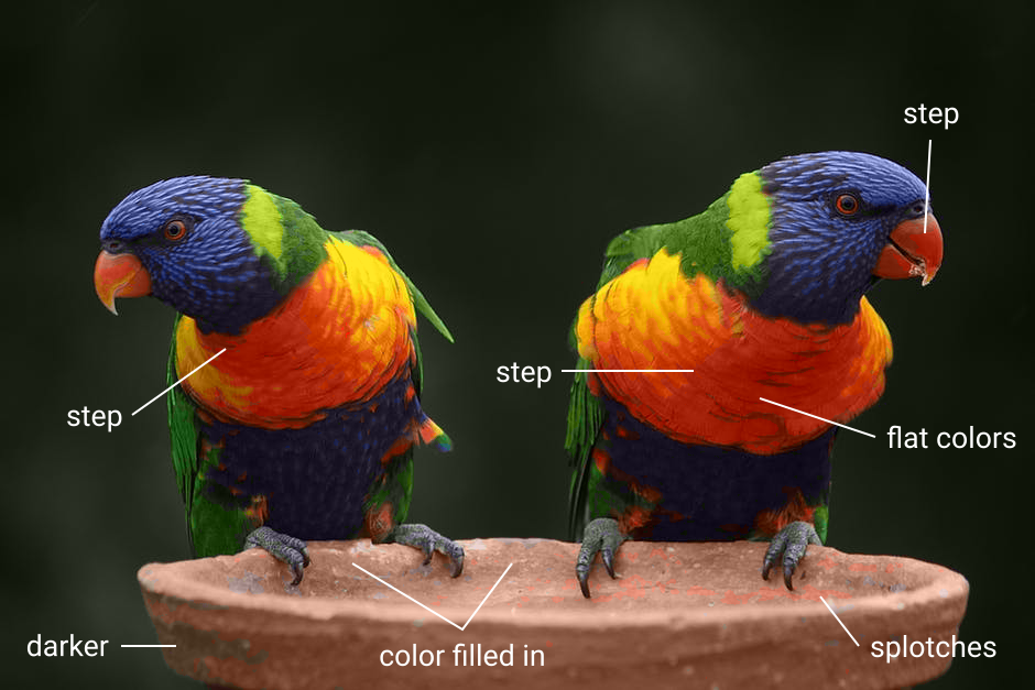
Reconstructed picture of parrots after applying quantization of 20 colors.
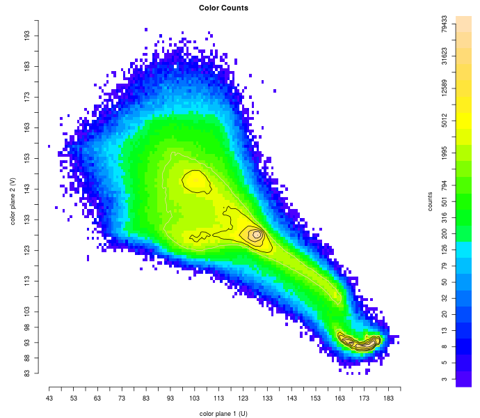
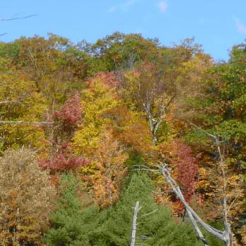
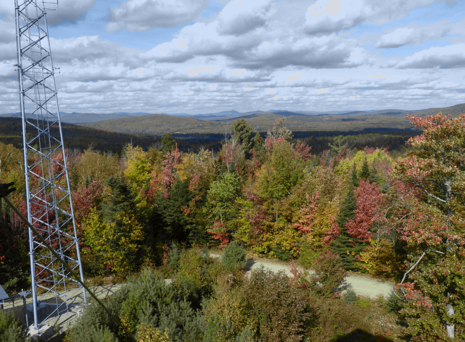
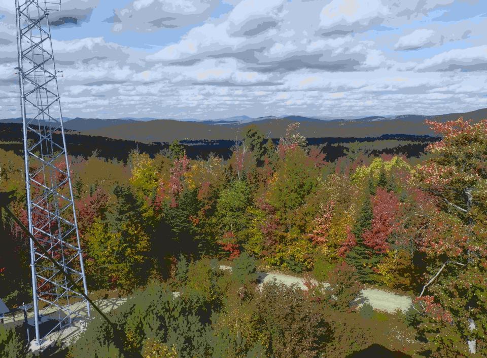
Our second example, which we used to demonstrate the need to limit a peak's extent, reduces the original colors to 19, plus 60 allocated on the peripheral grid. The histogram has large peaks around the grey value, blue for the sky and pond, and brown for the foliage. The rounded boundary to peaks 1 and 4 indicates the algorithm has limited the peaks' extent.
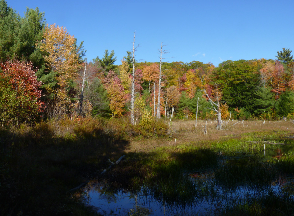
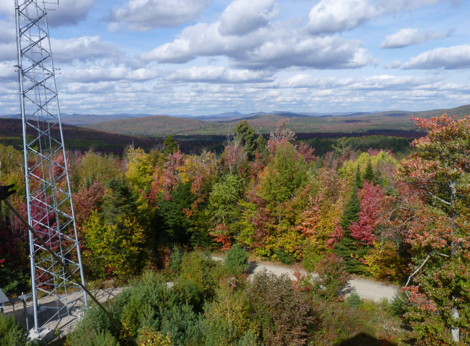
Second quantization example, a pond below Rose Mt. in fall.
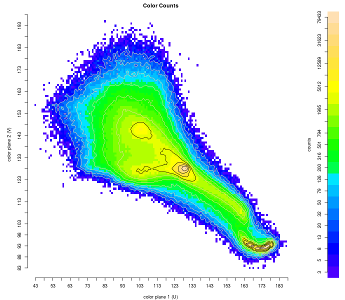
Height map of image's histogram.
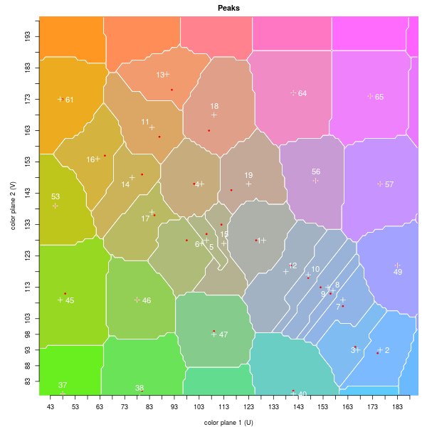
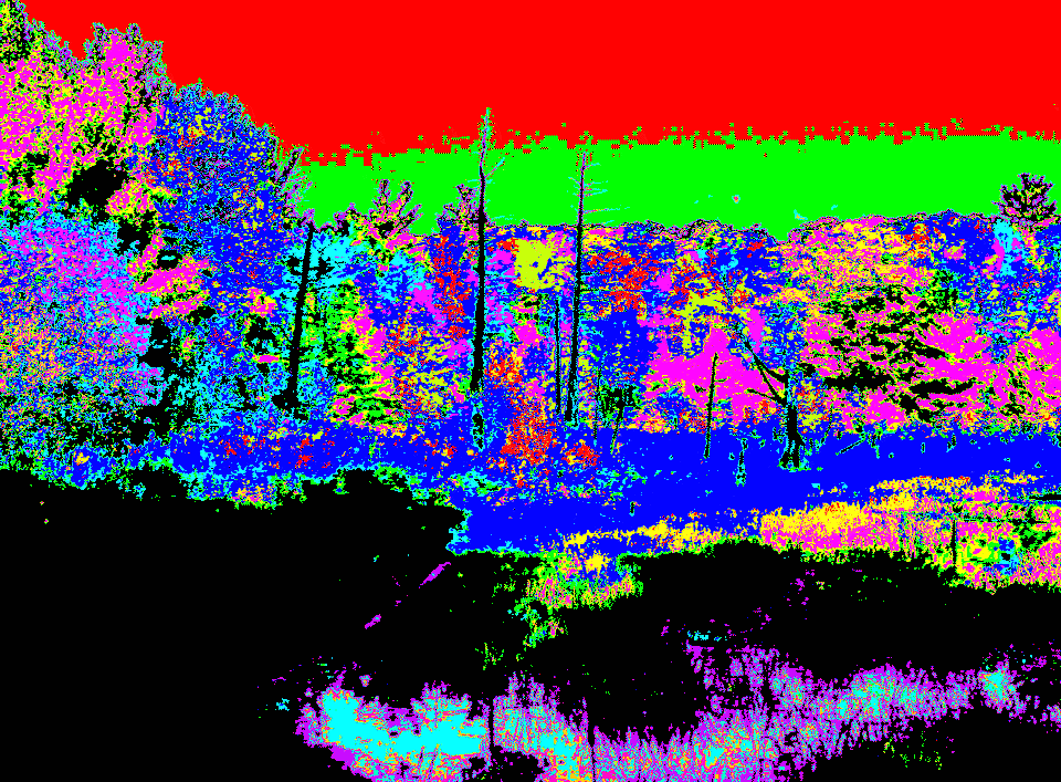
Quantization of pond. Graph on left shows peaks and corresponding color relative to the height map. Graph on right shows location of peaks (crosses) and centers of mass (dots). Bottom image has peak assignments, with random coloring.
The reconstructed image has no obvious mismatches. There is some blotchiness in the branches of the dead tree furthest to the left; the brown in the grass around and in the pond is deeper; there is unevenness in the green in the bushes in the center; and small areas of red and yellow have been replaced by brown (also visible to the right side of the close-ups above). There is a light banding of the two sky colors, mitigated by the closeness of the centers of mass (IDs 2 and 3) and the rough edge between.

Reconstructed image of pond after quantizing to 19 colors.
This algorithm runs at frame rates on our systems. A 1.5 Mpix RGB image can be processed in 28.6 ms, needing 6.7 ms to convert to YCrCb, 2.2 ms for Step #1, 2.4 ms for #2 t/m #8, 4.4 ms for #9 and #10, and 12.9 ms to build the reverse map and convert quantized colors back to RGB. The color conversion, region grow in Step #9, and mapping can be done on a GPU, cutting the time to 22.2 ms. The core timing depends on the color complexity of the scene, since the number of bins is fixed at 256x256: for the parrots (0.6 Mpix) we get 1.6 ms for Step #1, 4.9 ms for #2 t/m #8, and 5.6 ms for #9 and #10 (12.1 ms total), and for the pond (2.7 Mpix) it's 3.1 ms for #1, 4.1 for #2 t/m #8, and 4.9 for #9 and #10 (12.1 ms in total).
We have separated out the luminance from color channels. It too can be quantized, either together with the color plane, which requires a 3D watershed, or separately, as a 1D problem. The same approach of using a histogram of pixel counts works, and it is enough to have local minima separate quantization regions. Again there is a question of what defines a subsidiary peak that will merge into a neighbor. In general, although one can significantly reduce the number of greyscale values, in the process one loses too much detail and reconstructed images will have flat, colored areas similar to rotoscoping.
Luminance and color quantization from original image (top), color only (bottom left, to 15 colors), both (bottom right, to 9 greys). Color quantization has little color in mid-ground and areas of grey in the sky; saturated clouds are from clipping during color conversion. Luminance quantization creates areas of flat color in sky, mid-ground, and trees at bottom of image.
The biggest open question we have about this approach is, how stable are the results? Can they be used to characterize a scene, or do peaks drift under different lighting conditions, perhaps the time of day or year or weather changes, or between different cameras? We have tried many other quantization techniques, including k-means and DBSCAN clustering, mean cut algorithms, and Gaussian mixture models, and have found problems with all, including their performance, complexity and speed, and the assumptions they make. Right now the watershed algorithm is our go-to method to simplify the colors in an image.
The parrots picture is by Pixabay and found on Pexels. Other images are from PMVS.