Spacing and Multi-Modality
Introduction to Spacing and Modality Detection
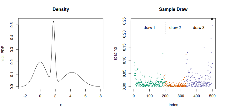
When looking at a histogram of data we often wonder if separate bulges in the counts represent different processes at work, or if they are just statistical fluctuations in a single process. Higher counts within a histogram bin implies a smaller separation between the data points, assuming they are spread equally over the bin's width. Fewer counts between the bulges correspond to larger separations. These separations are the spacing of the data, defined as the difference between consecutive order statistics or more simply after sorting.
Tri-modal setup and spacing in sample draw.
Consider this example. The histogram or total density function on the left shows a narrow peak between two others, and the rightmost is the widest. This is a tri-modal setup, built from three normal variates. The modes fall at the means, located at 0, 1.75, and 4.2, and the width of each depends on the standard deviation, 0.8, 0.2, and 1.2. We make a sample draw from each, of 200, 125, and 175 points, and plot the spacing on the right. A few features appear. The spacing is consistent within each variate, with the smallest values in the narrow variable in the middle and largest values to the right; this follows the widths. There are a few large spacings at the transition between the draws, near indices 200 and 325. The spacing also increases strongly at the start and end of the data, especially on the right side where two points with values of 0.302 and 0.480 fall outside the graph. Finally, although the spacing is consistent for each variate, it is not a constant, and we see a fair amount of noise or point-to-point variation.
Spacing allows us to say not just if there is more than one mode, but to locate them. Our approach will work with data taken to only a few decimal places, or even integers, which creates steps at new values and is zero for ties. Local increases in the spacing provide the best indication of multi-modality, lying at the anti-modes. Consistent or flat sections estimate the modes.
Spacing is not a new concept, with known formulas for its density based on the distribution of order statistics. The expected value and variance follow from the moments of this density. These can be solved for only a few cases. Uniform and exponential variates have simple forms. We have been able to do the integrals for logistic and Gumbel variates, and have found that the derivative of the inverse cumulative density function, also called the quantile function, is an estimator of the expected spacing. Other distributions and combinations of more than one variate do not have closed-form expressions and can only be evaluated numerically, which provides little insight into how the features, those local increases between modes and the stable values within, will behave. In general the expected spacing takes the form of a 'U', increasing sharply in the tails from a broad base. The leading and trailing increases will obscure the effect of mode changes (a favorite stress test in the literature), but within the base the features will be clear.
Our paper "Expected Spacing" describes the estimator and the new logistic and Gumbel solutions. Its supplement works out the integrals, performs additional error analysis of the estimator, and describes the data files used to generate the figures. A second paper, "A Spacing Estimator", adds the spacing's variance for logistic variates. The series solutions for the new solutions require a high-precision math library like mpfr because they have terms that nearly cancel, and three programs provide reference implementations for the calculations.
Detecting and Evaluating Features
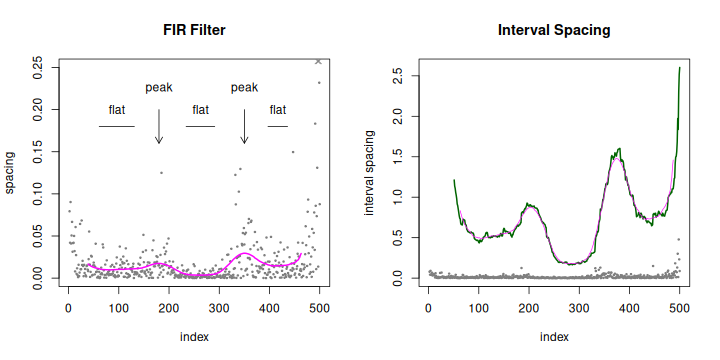
The features in the spacing are what we need to detect and analyze if we are to use spacing to identify modes within the data. The high noise level means that some sort of low-pass filtering will be needed, and the features will appear as peaks or flats. A finite impulse response filter (FIR) like the Kaiser kernel works well.
Sometimes the difference in order statistics over a gap has been used, as an estimator of the mode or to detect portions of the data with non-zero slope. We call this the "interval spacing". Using the standard notation from Pyke, if the spacing at index and order statistic , then the interval spacing for a gap of width . Once again the density of Diw is known and solved for uniform and exponential variates. Our paper "Interval Spacing" adds a series solution for logistic variates, with the supplement working out all integrals. It also shows that Diw is the sum of the spacings over the interval. But this is equivalent to a rectangular FIR filter, or running mean. Normally this is considered a poor low-pass filter. Although its mainlobe is wide, so that the kernel width can be smaller, it has large sidelobes which will leave high-frequency components. The interval spacing will be rough, making feature detection more difficult but also allowing some additional opportunities for testing. When comparing the filtered signals, you must account for the two indexing schemes (the FIR kernel is centered, the interval spacing lies at the upper edge) and amplification of Diw, which does not scale by the width. In our example the Kaiser response has been shifted and scaled to align with the interval spacing, whose roughness in comparison is clear.
Tri-modal spacing after Kaiser low-pass filter (left) or interval spacing (right).
The features are simple. Peaks are local maxima, with larger values than either neighbor. The detector treats small differences as equal values so that rough tops collapse to a point. It merges small subsidiary peaks into larger, similar to ignoring knobs on a ridge falling away from a mountain top. Flats are defined by a ripple specification so their height is a fraction of the signal's range. We characterize peaks by their height above the minima to either side. Since the ripple fixes a flat's height, its characteristic value is its length.
In the low-pass tri-modal example there are peaks at indices 180 and 350. Flats are found at the three troughs, 61–131, 234–291, and 397–436. Note that the flat mid-points are shifted slightly from the middle of the draws, and the peaks do not lie at the boundaries of the draws. Capturing such interactions between the variates is what we lose by not being able to solve or model the combined expected spacing. The peaks inside the interval spacing for the first draw, at indices 116 and 150, are merged because they are small.
How do we evaluate the features we find, to determine if they really correspond to modes and anti-modes? Our tests developed to minimize assumptions. We started with parametric models, turned to runs within the interval spacing for non-parametric checks, tried data-based simulations of the features, and finally used changepoint detectors.
1. Parametric Models
To build the models we run the feature detectors on a very large number of draws from a single null distribution, gathering their size as we change the sample size and filter width. The model links the critical values, the peak height or flat length, against the quantiles over all draws for each combination of the sample size and filter.
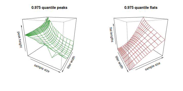
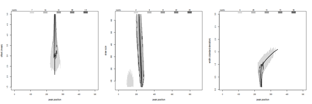
Peak height (left) and flat length (right) as null draw size and filter width change.
In a way the two models are complementary. The peaks have a clear conservative choice for the null distribution, an asymmetric Weibull variate whose critical heights at the 0.95 quantile are the same as other variates at the 0.975 or 0.99 level. The relationship between the length and three dependent variables is complicated, however, and is best fit as a Wald distribution. The fit becomes poor for small samples of 70 or fewer points, and uncertain for quantiles beyond 0.999. The flat model is much simpler and fits the simulated quantiles well over the parameter space, but the null distribution is much less obvious. There is a large spread in the critical lengths from any distribution, and little overlap between nulls. The default choice, a logistic variate, is a compromise.
The models test compares the height of peak above its bounding minima, or the length of a flat, to the quantile distribution given the sample size, filter, and for flats the null variate.
2. Runs Tests
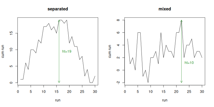
The parametric models after low-pass filtering are equivalent to bump-hunting after kernel density estimation, an approach that has been used by others to study modality, although not with the fits we have made. To remove the dependence on the null distribution we next looked at runs. We convert the interval spacing into three symbols by taking the sign of the difference between adjacent points - the interval spacing increases, decreases, or remains tied. We can then study sequences of same symbols within a feature. This approach has been used in economics to look at rising or falling trends in prices, or in cards to get the probability of various hands. Converting a signal into its signed difference generally preserves the shape, amplifying small differences and compressing large if their scaling does not match the length of the run. Within a feature, for example a peak bounded by the surrounding minima, we could test any number of quantities: how many runs there are, the distribution of their length, or the longest.
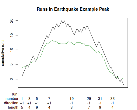
Runs (black) in the signed difference of the interval spacing.
Kaplansky and Riordan used combinatorial counting to show that the number of runs within a draw is distributed normally, with mean and variance depending on the number of each symbol. The runs count (nrun) test compares the actual number of runs to the expected.
The combinatorial counting ignores any correlations between symbols introduced by filtering. We have modeled the runs using a Markov chain based on the actual transitions between symbols, and have solved for the probability of getting a run of a given length,
where is the stationary state of the chain or a unit vector if starting from a known state and is a recursion
with seed
.
is the diagonal of the chain's transition matrix that advances a run within each symbol, and the off-diagonal elements that reset back to a new run. The runs length (runlen) test builds the transition and stationary state matrices from the complete interval spacing and calculates the probability of the longest run within a peak.
3. Data-Driven Tests
A final check that can be done with runs is to ask, how often they can re-create the feature? That is, we permute the runs within the feature, re-create the height for each permutation, and compare the actual height to this distribution to get its probability. The permutations must alternate symbols — we cannot place two increasing series next to each other or they would form a longer single run that does not exist in the data. The idea is that the longest runs must separate, rising at the start of the permutation and falling later, to get a large peak. If they mix then the height will be small. The runs height (runht) test or runs permutation test returns the probability of the peak as the fraction of simulated heights below the actual. If there are too many permutations to exhaustively enumerate then we sample a subset.
Permutations re-create a peak if long runs are separated (left).
We can extend this approach to arbitrary data by using the local differences in the signal as the pool to sample from, rather than permuting a set of runs. This is a bootstrap and sampling is done with replacement. The re-created feature is the cumulative sum of the drawn differences, and again we compare the feature's height to the fraction of the bootstraps yielding a smaller height. We need to exclude the large differences from the tail of expected spacing, in the arms of the 'U' at the ends of the data, because they do not represent the signal, but keep all differences, however large, in the middle.
The excursion test works with both peaks and flats, whose probability will be the number of bootstrap samples with height smaller or larger than the feature's.
4. Changepoints
As a final check of the spacing, we turn to the rich field of changepoint detectors. These look where the spacing changes its behavior at the transition between mode and anti-mode. Changepoint detection has its roots in statistical process control and economic trend analysis, and there are more than 25 packages available in R. The algorithms are truly varied: two-sample tests to identify changes in the mean or variance; cumulative sums to amplify trends; parametric models to mark outliers; segmentations of consistent values based on information or entropy criteria; Bayesian models; the breakdown of regression fits.
Changepoints by majority voting.
We remain agnostic about which detectors should be used. Instead, we treat this as a problem in classifier fusion, or combining the results of whichever detectors are available. We use a majority voting scheme, treating slightly shifted changepoints as the same before counting how many detectors identified the point.
Unlike the peaks and flats, changepoints will not usually match features. If the edge is sharp, like the middle variate in the tri-modal example, then the changepoint will lie close to the endpoint of a flat or to a peak, but more often it will fall to the side. There is no way to assess the quality of the changepoint, since few detectors provide a significance estimate for their results and the voting is really combining only yes/no decisions. The detectors are sensitive to the large spacings at the start and end of the data and often identify changepoints there. They also do badly with quantized data, reacting to each new value rather than picking up changes in how often they occur.
For these reasons changepoints will complement the feature analysis. They may indicate multi-modality but do not locate the modes well.
Implementations and Performance
The R package Dimodal, available here or on CRAN, provides the reference implementation of the feature detectors and tests. The technical report for the project describes the development of the models and has a complete evaluation of the test performance. Limitations in the platform for handling optional packages mean the CRAN version does not include the changepoint analysis.
We have ported the package to a stand-alone C program, DimodalC, and used SWIG to create bindings to it for a Python version, DimodalPy. The source code for both is available here. DimodalC has been compiled and tested under both Linux and Windows, and DimodalPy only under Linux. A Linux binary distribution for DimodalPy is available here. The README files provided with the source code will tell you how to use these versions. The port does simplify the code, removing some functionality and tweaking the behavior of the detectors and tests.
We can use a simple bi-modal setup to study how spacing reflects multi-modality. We combine draws from two normal variates, varying one parameter of the second — its mean or separation to the first, its standard deviation or width, or the draw size. We expect that peaks and flats will fall at the anti-mode or modes until it becomes hard to distinguish the two, for small separations or large widths.
Peak positions for bi-modal variants.
For peaks we plot greyscale-encoded histograms of their location over 1000 trials of each variant, changing the mean in the left graph, the draw size in the middle, and the standard deviation in the right. The thick solid line marks the ideal anti-mode, found by numerically integrating the expected spacing for the variant. It disappears in the numeric solution when the draws cannot be separated, for a mean smaller than 2.4 or width larger than 1.5. The contour line includes the peaks passing either the height model or excursion test, while grey areas outside represent detected peaks that are not accepted. The outer grey level extends along the line almost to its end so the spacing can in principle resolve even close modes, although its widening means the peak position becomes less stable or more uncertain. The accepted features stay back from the end, reaching to a mean of 3.0 or standard deviation of 1.0. They stay close to the anti-mode. The peaks are insensitive to changes in the draw size, except that a second appears in the first variate when it is much larger. Testing rejects these.
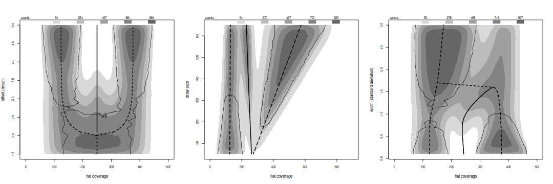
Flat spans for bi-modal variants.
The histograms for flats count how many span each point; because flats can overlap the graphs may not reflect individual features and counts will be higher. They cover the modes, separately when there are significant peaks but merging as the variates grow indistinguishable. The transitional peaks are often large enough to support some flats, seen as fingers along the anti-mode line in all three graphs. Tests reject these and marginal flats away from the modes in the width and draw size variants. They accept flats in the larger mode when the draw sizes are unbalanced, or both if the sizes are within 50 points.
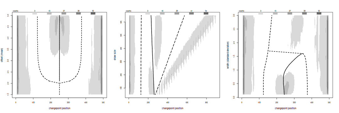
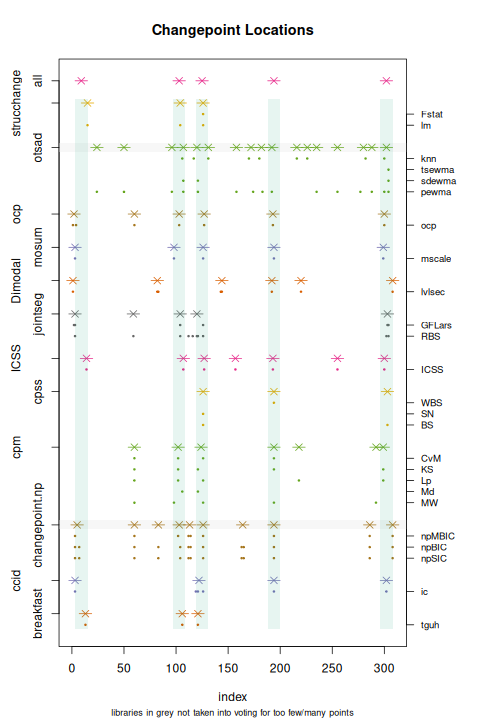
Changepoint locations for bi-modal variants.
Changepoints when they occur fall to the side of the anti-mode. They resolve fewer variates, needing separations above 3.3 or standard deviations below 0.9, and trigger at the edge of the larger draw. The strongest counts are pinned to the edges of the data, caused either by the large spacing in the tails or by the start-up of the detectors, which usually use 15 or 20 points to provide a base reference for their analysis.
In summary, detected peaks follow the anti-mode, although they become less stable as the variates begin to merge. Testing keeps peaks close to the anti-mode, providing an accurate, repeatable estimate of its location. Flats follow the modes. Testing rejects those appearing away from a mode.
To see how effective each test is, we perform a row sum across the greyscale histograms for each variant, giving the uni-modal rate as the number of trials that do not have a peak passing that test.
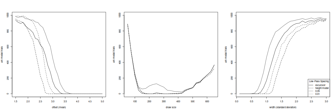
Modality resolution by low-pass test and acceptance level for bi-modal variants.
In the low-pass spacing the height model at its recommended acceptance level (0.01, light dashed curve) has a sharp transition at a separation of 2.6, but has a slow ramp for large standard deviations, above 1.5, which will generate false positives. Loosening the acceptance level (0.05, dark dashed curve) resolves the anti-mode until it almost disappears but exacerbates the false positive problem. The excursion test at its recommended level (0.05, dark solid curve) is a little less sensitive than the model, and does not have a sharp transition for small means. A tighter level (0.01, light solid curve) will remove these false positives, but will also require the variates be more distinct, by a shift in the mean of 0.3 or in the standard deviation by 0.2. Both tests start to lose resolution when the draws are very unbalanced; the curves in the middle graph would be more symmetric were we to plot the rates against the ratio of the two draws. Both tests perform like the excess mass test for modality and are more sensitive than the dip and critical bandwidth tests, and have the advantage of checking peaks separately, allowing us to assess individual anti-modes.
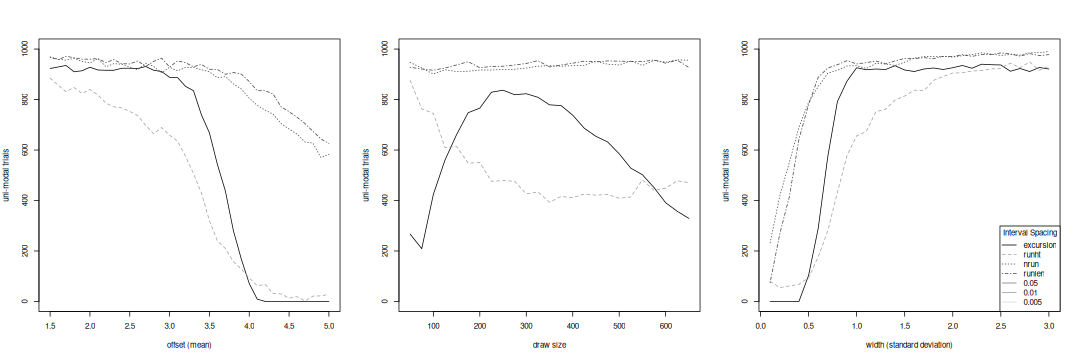
Modality resolution by interval spacing tests for bi-modal variants.
The two runs tests in the interval spacing perform very much alike. They are insensitive, requiring very large offsets or a very narrow second draw before they respond. The transition is sharp for the standard deviation but not for the mean. A pass for these tests should be a strong consideration for an anti-mode, but other tests will likely pass first. The draw size variants show no response because their default mean and width are below what the tests can resolve. The run permutation test resolves offsets above 3.5 or widths below 0.8. Both variants show slow transitions, even with a very tight acceptance level, so false positives can be a problem. The excursion test makes a cleaner decision, but requires a minimum offset of 3.7 or maximum standard deviation of 0.7. The default conditions for the draw size variations mean the run height test only partially resolves the variates, and that the excursion test actually has an easier time distinguishing unbalanced draws.
There is little correlation between the individual tests. We can therefore take them as an ensemble, with any accepted result flagging an anti-mode. We control the overall false positive rate with individual thresholds, chosen conservatively rather than for maximum sensitivity. We find many more peaks in the interval spacing thanks to its roughness, but the lower test sensitivity equalizes the number accepted. The alignment between spacings is loose due to the roughness.
An Example
D. W. Scott collected the depth of 510 earthquakes below Mount St. Helens before its eruption. Magma collected in a reservoir 12 to 7 km below the mountain and fed to the summit crater through a 50 m conduit to the surface vent system. Starting in March, 1980 most earthquakes occurred at the top of the conduit and the vent system, but there was also seismic activity in the reservoir. Do we see this separation in the data?
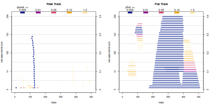
Tracking plot of peaks (left) and flats (right) as low-pass filter size changes.
To begin the analysis we generate a tracking plot that varies the size of the low-pass filter and plots the location of the features. This is similar to a mode tree or SiZer graph. Peaks are marked with dots that are filled in if any test passes its acceptance level, and flats are marked over their span. Both are color-coded by the best test probability. We see in the graph that we need a small window of 0.08 to pick up a second weak peak near index 400, but a strong, significant peak persists above index 100 over the usual filter size range, 0.05 – 0.20. The weak peak separates two strong flats, so we will chose to do the analysis with this window. We will leave the interval spacing at its default value, 0.10.
> library(Dimodal)
> data(earthquake, package="feature")
> trk <- Ditrack(earthquake$depth)
> dev.new(width=10,height=5) ; plot(trk)
Dimodal uses an options database similar to par() to set parameters for the feature detectors, tests, their acceptance levels, and for displaying results. Diopt() sets the values globally while Diopt.local() provides one-time overrides. We do not need to change any parameters except the window size.
> Diopt(lp.window=0.08)
Like par(), this returns the old values for the changed parameters. Typing Diopt() at the command prompt will return the whole database.
Run the modality analysis with
> m <- Dimodal(earthquake$depth)
We look at the results with
> dev.new(width=15,height=5) ; plot(m)
which creates three graphs. The histogram in the middle shows most quakes happen within 2 km of the surface, with the highest count at the surface. The reservoir is also clear.
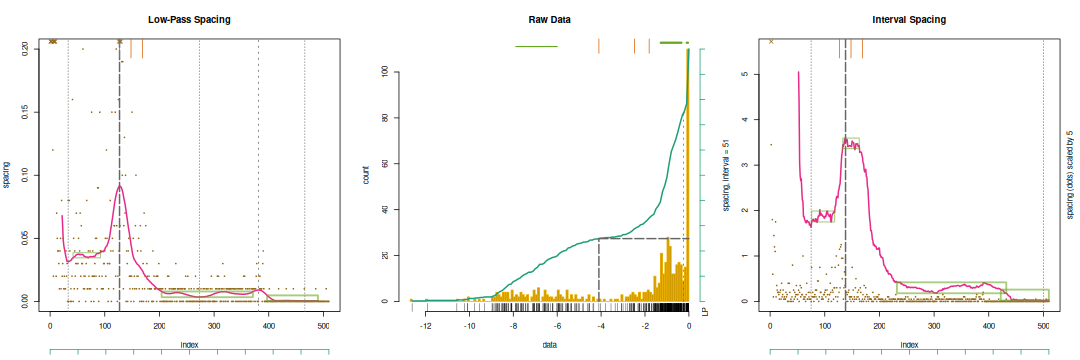
Spacing analysis of earthquake depth under Mt. St. Helens.
The left graph has the low-pass filtered results. The dots mark the raw spacing values, and it is clear that the data is quantized — depths were taken to two decimal places, so any difference between two points is a multiple of 0.01. The red curve is the smoothed spacing. There is an obvious peak at index 127 and a weak one at 381; both are marked with dashed lines. The dotted lines give the local minima. Boxes surround the flats, between indices 42 and 92, 204 and 371, and 397 to 490. Heavy marks mean the feature has passed at least one test. The long tick marks at the top of the graph are the common changepoints, and trigger at the large peak and to its right.
These marks also appear in the histogram, with bars at the top replacing the boxes for flats. The axes below the spacings or to the right of the histogram give deciles. When combined with the cumulative distribution drawn atop the histogram they convert between the index in the spacing and raw data values, as the peak mark demonstrates.
Looking at the test results,
> m$lp.peaks
location of maxima
pos raw minima pos (raw) support pos
127 (-4.100) 33 - 273 ( -8.2300 - -0.91143) 85 - 191
381 (-0.248) 273 - 466 ( -0.9114 - -0.05439) 286 - 407
statistics
pos ht hexcur
127 3.9782 0.079222
381 0.3893 0.007563
probabilities
pos pht pexcur ppeak pass
127 _0.0000_ _0.0000_ 0.0000 T (2)
381 0.2909 0.8175 0.2909
accept at
0.0100 0.0500
The large peak at index 127 corresponds to a quake depth of -4.1 km and passes both the height model and excursion test, as flagged by the surrounding underscores. The weak peak at index 381 separates the surface and shallow quakes at -0.25 km but is not large enough to pass either test.
> m$lp.flats
statistics
endpoints raw len hexcur
42 - 92 (-7.88333 -6.0000) 51 0.004077
204 - 371 (-1.28250 -0.3400) 168 0.004505
397 - 490 (-0.09889 -0.0425) 94 0.004393
probabilities
endpoints plen pexcur pflat pass
42 - 92 0.6685 0.0531 0.0531
204 - 371 0.0590 _0.0001_ 0.0001 T (1)
397 - 490 0.3890 _0.0026_ 0.0026 T (1)
accept at 0.0500 0.0100
The first flat, covering the top of the reservoir, is too short to pass either the length model or excursion test. The other two pass the excursion test, with the second also narrowly failing the length model.
The interval spacing results in the right graph are similar: one large peak between the reservoir and conduit, and two flats separating the surface vent system from the conduit. The roughness of the interval spacing compared to the Kaiser filter is clear. It leads to uncertainty in the peak's position, shifting the depth to -5.2 km. The peak passes all runs tests except the longest run, which gives a marginal result. The weak peak at index 381 is too small for the detector and is merged into the main peak. Note that this pushes the minimum almost to the end of the data, and this would distort the peak width, since it incorporates two flats. The excursion test uses a smaller support for the feature, taking its width to some fraction of its height, by default 90%; this is the same that's done with Full Width at Half Maximum (FWHM). The range of support indices is half that between the minimum.
> m$diw.peaks
location of maximum
pos raw minima pos (raw) support pos
138 (-5.2) 75 - 500 (-7.64 - -0.05) 113 - 242
statistics
pos hexcur nrun runlen runht
138 3.22 231 13 67
probabilities
pos pexcur pnrun prunlen prunht ppeak pass
138 _0.0001_ _0.0000_ 0.0304 _0.0001_ 0.0000 T (3)
accept at
0.0500 0.0100 0.0100 0.0050
The two long flats in the conduit and vent system, between indices 232 and 432 (depth -1.27 to -0.09 km) and 422 and 510 (-0.10 and -0.05 km), pass the excursion test, while a flat between 42 and 92 (-7.88 and -6.00 km) does not. These flats match those in the low-pass spacing. At smaller intervals the roughness in the left flat would be large enough to create a detected peak.
To see the voting behind the changepoints you can run
> dev.open(width=5, height=10) ; plot(m$cpt)
The results will depend on which libraries you have installed on your system. Here we find three, at depths of -4.10 km, -2.48 km, and -1.81 km.
Scott's original analysis of this data used a logarithmic scaling of the depth to separate the conduit from the surface vent system. If you do this you will find two large peaks that pass testing, quantization of the shallowest depths that produce spurious peaks in the interval spacing, and an overall much rougher interval spacing. There will still be three flats, although only the one for the conduit would be significant.
For a second example the Dimodal package includes the kirkwood data set with the orbital axis of asteroids in the main belt. Here anti-modes correspond to the Kirkwood gaps, where regular perturbation by Jupiter moves asteroids away from the resonance into different orbits, and modes help to define families of asteroids that have a common origin. The example on the help page for the data set shows how to perform the analysis.